Everything Fibonacci

Sun Oct 07 2018

If you have ever taken a computer science class you probably know what the fibonacci sequence is and how to calculate it. For those who don’t know: Fibonacci is a sequence of numbers starting with 0,1 whose next number is the sum of the two previous numbers. After having multiple of my CS classes give lectures and homeworks on the Fibonacci sequence; I decided to write a blog post going over the 4 main ways of calculating the nth term of the Fibonacci sequence. In addition to providing the python code for calculating the nth perm of the sequence, a proof for their validity and an analysis of their time complexities both mathematically and empirically will be examined.

1 Slow Recursive Definition

By the definition of the Fibonacci sequence, it is the most natural to write it as a recursive definition.

def fib(n):
    if n == 0 or n == 1:
        return n
    return fib(n-1) + fib(n-2)

##Time Complexity

Observing that each call has two recursive calls we can place an upper bound on this function as \(O(2^n)\). However, if we solve this recurrence we can place a tight bound for time complexity.

We can write a recurrence for the number of times fib is called:

\[ F(1) = 1\\ F(n) = F(n-1) + F(n-2)\\ \]

Next, we replace F(n) with \(a^n\) since we want to find rate of exponential growth.

\[ a^n = a^{n-1} + a^{n-2}\\ \frac{a^n}{a^{n-2}} = \frac{a^{n-1} + a^{n-2}}{a^{n-2}}\\ a^2 = a + 1\\ a = \frac{1 \pm sqrt(5)}{2}\\ \]

From this calculation we can conclude that F(n) \(\in \Theta 1.681^n\). We don’t have to worry about the negative root since it would not be asymptotically relevant by the definition of \(\Theta\).

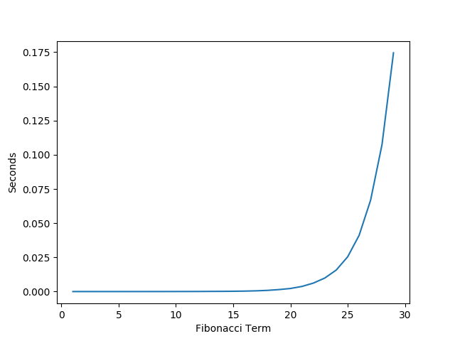
1.1 Measured Performance

Here is a graph of the actual performance that I observed from this recursive definition of Fibonacci.

2 Accumulation Solution

The problem with the previous recursive solution is that you had to recalculate certain terms of fibonacci a ton of times. A summation variable would help us avoid this problem. You could write this solution using a simple loop or dynamic programming , however, I chose to use recursion to demonstrate that it’s recursion which made the first problem slow.

def fibHelper(n, a, b):
    if n == 0:
        return a
    elif n == 1:
        return b
    return fibHelper(n-1, b, a+b)        

def fibIterative(n):
    return fibHelper(n, 0, 1)

In this code example, fibHelper is a method which accumulates the previous two terms. The fibIterative is a wrapper method which sets the two initial terms equal to 0 and 1 representing the fibonacci sequence. At first it may not be obvious that fibIterative(n) is equivalent to fib(n). To demonstrate that these two are in fact equivalent, I broke this into two inductive proofs.

2.1 Proof for Fib Helper

Lemma: For any n \(\epsilon\) N if n \(>\) 1 then \(fibHelper(n, a, b) = fibHelper(n - 1, a, b) + fibHelper(n - 2, a, b)\).

Proof via Induction

Base Case: n = 2: \[ LHS = fibHelper(2, a, b)\\ = fibHelper(1, b, a + b) = a + b\\ RHS = fibHelper(2 -1, a, b) + fibHelper(2-2, a, b)\\ = a + b\\ \]

Inductive Step:

Assume proposition is true for all n and show n+1 follows.

\[ RHS=fibHelper(n+1;a,b)\\ = fibHelper(n;b,a+b)\\ =fibHelper(n-1;b,a+b) + fibHelper(n-2;b,a+b)\\ =fibHelper(n;a,b) + fibHelper(n-1;a,b)\\ =LHS\\ \]

\(\Box\)

2.2 Proof That fibIterative = Fib

Lemma: For any n \(\in\) N, \(fib(n)\) = \(fibIterative(n, 0, 1)\)

Proof via Strong Induction

Base Case: n = 0: \[ fibIterative(0, 0, 0) = 0\\ = fib(0) \]

Base Case: n = 1: \[ fibIterative(1, 0, 0) = 1\\ = fib(1) \]

Inductive Step:

Assume proposition is true for all n and show n+1 follows.

\[ fib(n+1) = fib(n) + fib(n-1)\\ = fibHelper(n, 0, 1) + fibHelper(n+1, 0 ,1) \quad\text{I.H}\\ = fibHelper(n+1, 0, 1) \quad\text{from result in previous proof}\\ \]

\(\Box\)

2.3 Time Complexity

Suppose that we wish to solve for the time complexity in terms of the number of additions needed to be computed. Based on fibHelper we can see that it performs one addition every recursive call. We can now form a recurrence for time complexity.

\[ T(0) = 0\\ T(1) = 0\\ T(n) = 1 + T(n-1)\\ T(n) = n-1\\ \]

From this recurrence we can say that fibHelper \(\in \Theta(n)\).

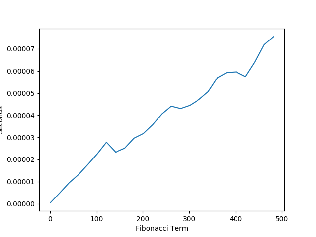
2.4 Measured Performance

Notice how much faster this solution is compared to the original recursive solution for Fibonacci.

3 Matrix Solution

We can actually get better than linear for performance for Fibonacci while still using recursion. However, to do so we need to know this fact:

\[ \begin{bmatrix} 1 & 1\\ 1 & 0 \end{bmatrix}^n = \begin{bmatrix} F_{n+1} & F_n\\ F_n & F{n-1} \end{bmatrix}^n \]

Without any tricks, raising a matrix to a power n times would not get us better than linear performance. However, if we use the Exponentiation by Squaring method, we can expect to see logarithmic time. Since two spots in the matrix are always equal, I represented the matrix as an array with only three elements to reduce the space and computations required.

def multiply(a,b):
    product = [0,0,0]
    product[0] = a[0]*b[0] + a[1]*b[1]
    product[1] = a[0]*b[1] + a[1]*b[2]
    product[2] = a[1]*b[1] + a[2]*b[2]
    return product

def power(l, k):
    if k == 1:
        return l
    temp = power(l, k//2)
    if k%2 == 0:
        return multiply(temp, temp)
    else:
        return multiply(l, multiply(temp, temp))

def fibPower(n):
    l = [1,1,0]
    return power(l, n)[1]

3.1 Time Complexity

For this algorithm, lets solve for the time complexity as the number of additions and multiplications required.

Since we are always multiplying two 2x2 matrices, that operation is constant time.

\[ T_{multiply} = 9 \]

Solving for the time complexity of fib power is slightly more complicated.

\[ T_{power}(1) = 0\\ T_{power}(n) = T(\left\lfloor\dfrac{n}{2}\right\rfloor) + T_{multiply}\\ = T(\left\lfloor\dfrac{n}{2}\right\rfloor) + 9\\ = T(\left\lfloor\dfrac{n}{2*2}\right\rfloor) + 9 + 9\\ = T(\left\lfloor\dfrac{n}{2*2*2}\right\rfloor) + 9+ 9 + 9\\ T_{power}(n) = T(\left\lfloor\dfrac{n}{2^k}\right\rfloor) + 9k\\ \]

let \(k=k_0\) such that \(\left\lfloor\dfrac{n}{2^{k_0}}\right\rfloor = 1\)

\[ \left\lfloor\dfrac{n}{2^{k_0}}\right\rfloor = 1 \rightarrow 1 \leq \frac{n}{2^{k_0}} < 2\\ \rightarrow 2^{k_0} \leq n < 2^{k_0 +1}\\ \rightarrow k_0 \leq lg(n) < k_0+1\\ \rightarrow k_0 = \left\lfloor lg(n)\right\rfloor\\ T_{power}(n) = T(1) + 9*\left\lfloor lg(n)\right\rfloor\\ T_{power}(n) = 9*\left\lfloor\ lg(n)\right\rfloor\\ T_{fibPower}(n) = T_{power}(n)\\ \]

Now we can state that \(fibPower(n) \in \Theta(log(n))\).

3.2 Inductive Proof for Matrix Method

I would like to now prove that this matrix identity is valid since it is not at first obvious.

Lemma: For any n \(\epsilon\) N if n \(>\) 0 then \[ \begin{bmatrix} 1 & 1\\ 1 & 0 \end{bmatrix}^n = \begin{bmatrix} F_{n+1} & F_n\\ F_n & F{n-1} \end{bmatrix}^n \]

Let

\[ A= \begin{bmatrix} 1 & 1\\ 1 & 0 \end{bmatrix}^n \]

Base Case: n = 1 \[ A^1= \begin{bmatrix} 1 & 1\\ 1 & 0 \end{bmatrix}^n = \begin{bmatrix} F_{2} & F_2\\ F_2 & F_{0} \end{bmatrix}^n \]

Inductive Step: Assume proposition is true for n, show n+1 follows \[ A^{n+1}= \begin{bmatrix} 1 & 1\\ 1 & 0 \end{bmatrix} \begin{bmatrix} F_{n+1} & F_n\\ F_n & F{n-1} \end{bmatrix}^n\\ = \begin{bmatrix} F_{n+1} + F_n & F_n + F_{n-1}\\ F_{n+1} & F_{n} \end{bmatrix}\\ = \begin{bmatrix} F_{n+2} & F_{n+1}\\ F_{n+1} & F_{n} \end{bmatrix}\\ \]

\(\Box\)

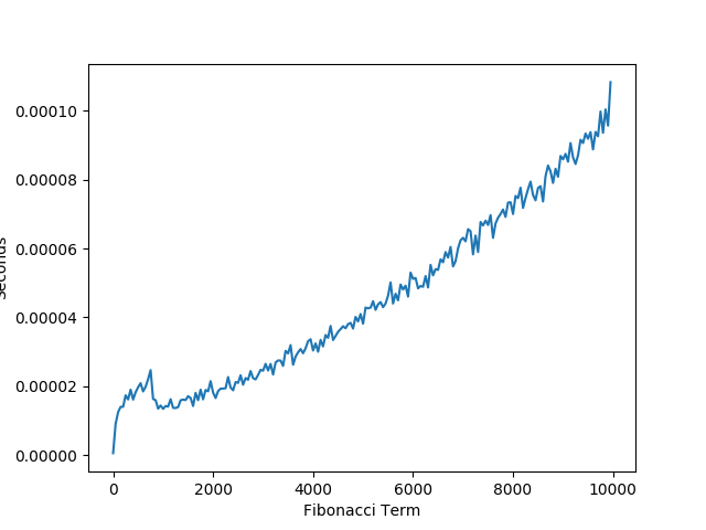
3.3 Measured Performance

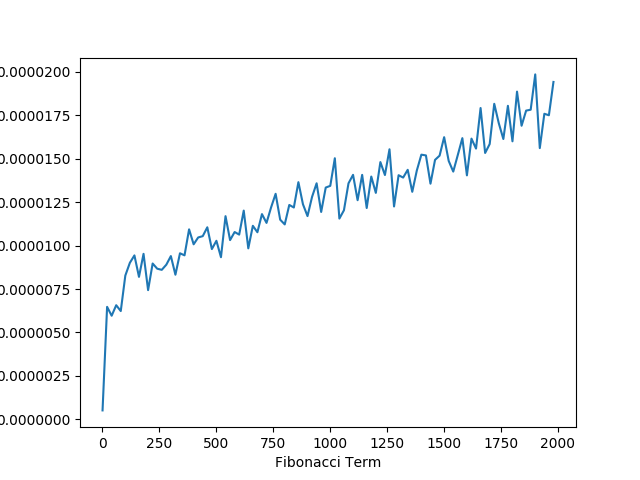
As expected by our mathematical calculations, the algorithm appears to be running in logarithmic time.

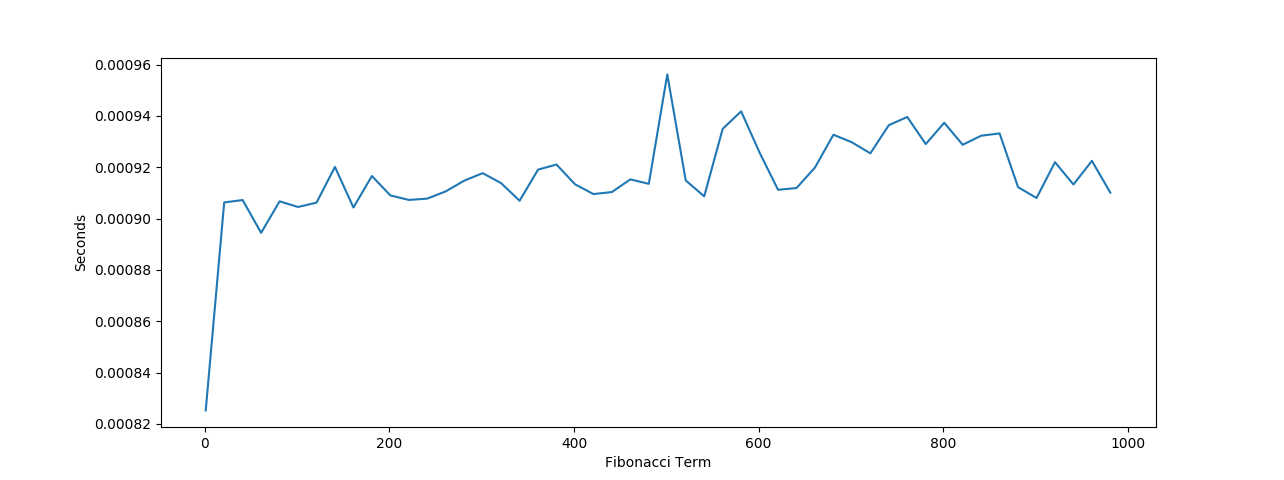
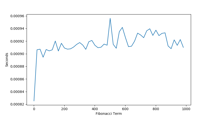
3.4 Measured Performance With Large Numbers

When calculating the fibonacci term for extremely large numbers despite having a polynomial time complexity, the space required to compute each Fibonacci term grows exponentially. Since our performance is only pseudo-polynomial we see a degrade in our performance when calculating large terms of the fibonacci sequence.

The one amazing thing to point out here is that despite calculating the 10,000 term of Fibonacci, this algorithm is nearly 400 times faster than the recursive algorithm when calculating the 30th term of Fibonacci.

4 Closed Form Definition

It is actually possible to calculate Fibonacci in constant time using Binet’s Formula.

\[ F_n = \frac{(\frac{1+\sqrt{5}}{2})^n-(\frac{1-\sqrt{5}}{2})^n}{\sqrt{5}} \]

def fibClosedFormula(n):
    p = ((1+ math.sqrt(5))/2)**n
    v = ((1-math.sqrt(5))/2)**n
    return (p-v)/math.sqrt(5)

4.1 Derivation of Binet’s Formula

Similar to when we were calculating the time complexity of the basic recursive definition , we want to start by finding the two roots of the equation in terms of exponents.

\[ a^n = a^{n-1} + a^{n-2}\\ \frac{a^n}{a^{n-2}} = \frac{a^{n-1} + a^{n-2}}{a^{n-2}}\\ a^2 = a + 1\\ 0 = a^2 - a - 1\\ a = \frac{1 \pm sqrt(5)}{2}\\ \]

Since there are two roots to the equation, the solution of \(F_n\) is going to be a linear combination of the two roots.

\[ F_n = c_1(\frac{1 + \sqrt{5}}{2})^n + c_2(\frac{1 - \sqrt{5}}{2})^n \]

Fact: \(F_1\) = 1

\[ F_1 = 1\\ = c_1(\frac{1 + \sqrt{5}}{2}) + c_2(\frac{1 - \sqrt{5}}{2})\\ = \frac{c_1}{2} + \frac{c_2}{2} + \frac{c_1\sqrt{5}}{2} - \frac{c_2\sqrt{5}}{2}\\ \]

Let \(c_1 = \frac{1}{\sqrt{5}}\), Let \(c_2 = \frac{-1}{\sqrt{5}}\)

\[ F_n = \frac{1}{\sqrt(5)}((\frac{1+\sqrt{5}}{2})^n-(\frac{1-\sqrt{5}}{2})^n)\\ = \frac{(\frac{1+\sqrt{5}}{2})^n-(\frac{1-\sqrt{5}}{2})^n}{\sqrt{5}} \]

4.2 Time Complexity

Since we managed to find the closed form of the fibonacci sequence we can expect to see constant performance.

4.3 Measured Performance