Developing an AI to Play Asteroids Part 1

Wed Dec 18 2019

I worked on this project during Dr. Homans’s RIT CSCI-331 class.

1 Introduction

This project explores the beautiful and frustrating ways in which we can use AI to develop systems to solve problems. Asteroids is a perfect example of a fun learning AI problem because Asteroids is difficult for humans to play and has open-source frameworks that can emulate the environment. Using the Open AI gym framework we developed different AI agents to play Asteroids using various heuristics and ML techniques. We then created a testbed to run experiments that determine statistically whether our custom agents out-performs the random agent.

2 Methods and Results

Three agents were developed to play Asteroids. This report is broken into segments where each agent is explained and its performance is analyzed.

3 Random Agent

The random agent simple takes a random action defined by the action space. The resulting agent will randomly spin around and shoot asteroids. Although this random agent is easy to implement, it is ineffective because moving spastically will cause you to crash into asteroids. Using this as the baseline for our performance, we can use this random agent to access whether our agents are better than random key smashing – which is my strategy for playing Smash.

"""
ACTION_MEANING = {
    0: "NOOP",
    1: "FIRE",
    2: "UP",
    3: "RIGHT",
    4: "LEFT",
    5: "DOWN",
    6: "UPRIGHT",
    7: "UPLEFT",
    8: "DOWNRIGHT",
    9: "DOWNLEFT",
    10: "UPFIRE",
    11: "RIGHTFIRE",
    12: "LEFTFIRE",
    13: "DOWNFIRE",
    14: "UPRIGHTFIRE",
    15: "UPLEFTFIRE",
    16: "DOWNRIGHTFIRE",
    17: "DOWNLEFTFIRE",
}
"""
def act(self, observation, reward, done):
    return self.action_space.sample()

3.1 Test on the Environment Seed

It is always important to know how randomness affects the results of your experiment. In this agent, there are two sources of randomness, the first being the seed given for the Gym environment and the other is in the random function used to select a random action. By default, the seed of the Gym library is set to zero. This is useful for testing because if your agent is deterministic, you will always get the same results. We can seed the environment with the current time to add more randomness. However, this begs the question: to what extent does the added randomness change the scores of the game. Certain seeds in the Gym environment may make the game much easier/harder to play thus altering the distribution of the score.

A test was derived to compare the scores of the environment in both a fixed seed and a time set seed. 300 trials of the random agent were ran in both types of seeded environments.

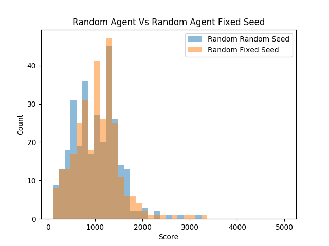
Random Agent Time Seed: 
    mean:1005.6333333333333 
    max:3220.0 
    min:110.0 
    sd:478.32548077178114 
    median:980.0 n:300

Random Agent Fixed Seed: 
    mean:1049.3666666666666 
    max:3320.0 
    min:110.0 
    sd:485.90321281323327 
    median:1080.0 
    n:300

What is astonishing is that both distributions are nearly identical in every way. Although the means are slightly different, there appears to be no apparent difference between the distributions of scores. One might expect that having more randomness would at least change the variance of the scores, but none of that has happened.

Random agent vs Random fixed seed
F_onewayResult(
    statistic=1.2300971733588375, 
    pvalue=0.2678339696597312
)

With such a high p-value we can not reject the null hypothesis that these distributions are statistically different. This is a powerful conclusion to come to because it allows us to run future experiments understanding that a specific seed on average will not have a statistically significant impact on the performance of a random agent. However, this finding does not help us understand the impact that the seed has on a fully deterministic agent. It is still possible that a fully deterministic system will have varying scores on different environment seeds.

4 Reflex Agent

Our reflex agent observes the environment and decides what to do based on a simple rule set. The reflex agent is broken into three sections: feature extraction, reflex rules, and performance.

4.1 Feature Extraction

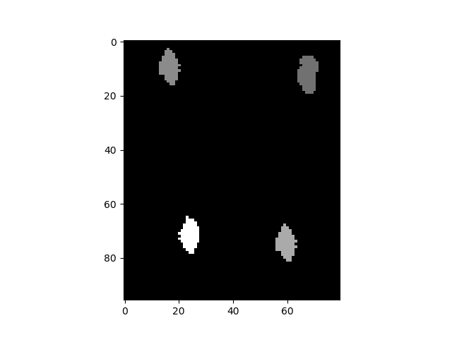
The largest part of this agent was devoted to parsing the environment into a more usable form. The feature extraction for this project was rather difficult since the environment was given as a pixel array and the screen flashed the asteroids and then the player. Trying to achieve the best performance with the minimal amount of algorithmic engineering, this reflex agent parsed 3 things from the environment: position, direction, closest asteroid.

4.1.1 1: Player Position

Finding the position of the player was relatively easy since you only had to scan the environment to find pixels of certain RGB values. To account for the flashing environment, you would just store the position in the fields of the class so that it is persistent between action loops. The position of the player would only be updated if a new player is observed.

AGENT_RGB = [240, 128, 128] 

4.1.2 2: Player Direction

Detecting the position of the player could be made difficult if you were only going off the RGB values of the player. Although when the player is upright, it is straight forward, when the player is sideways things get super difficult.

action_sequence = [3,3,3,3,3,0, 0,0]

class Agent(object):
    def __init__(self, action_space):
        self.action_space = action_space

    # Defines how the agent should act
    def act(self, observation, reward, done):
        if len(action_sequence) > 0:
            action = action_sequence[0]
            action_sequence.remove(action)
            return action
        return 0

We created a basic script to observe what the player does when given a specific sequence of actions. I was pleased to notice that exactly 5 turns to the left/right correlated to a perfect 90 degrees. By keeping track of our current rotation according to the actions that we have taken, we can precisely keep track of our current rotational direction without parsing the horrendous pixel array when the player is sideways.

4.1.3 3: Position of Closest Asteroid

Asteroids were detected as being any pixel that was not empty (0,0,0) and not the player (240, 128, 128). Using a simple single pass through the environment matrix, we were able to detect the closest asteroid to the latest known position of the player.

4.2 Agent Reflex

Based on my actual strategy for asteroids, this agent stays in the middle of the screen and shoots at the closest asteroid to it.

def act(self, observation, reward, done):
    observation = np.array(observation)
    self.updateState(observation)
    dirOfAstroid = math.atan2(self.closestRow-self.row, self.closestCol- self.col)

    dirOfAstroid = self.deWarpAngle(dirOfAstroid)

    self.shotLast = not self.shotLast
    if self.shotLast:
        return 1 # fire
    if self.currentDirection - dirOfAstroid < 0:
        self.updateDirection(math.pi/10)
        if self.shotLast:
            return 12 # left fire
        return 4 # left
    else:
        self.updateDirection(-1*math.pi/10)
        return 3 # right

Despite being a simple agent, this performs well since it can shoot at asteroids before it hits them.

4.3 Results of Reflex Agent

In this trial, 200 tests of both the random agent and the reflex agent were observed while setting the seed of the environment to the current time. The seed was randomly set in this scenario since the reflex agent is fully deterministic and would perform identically in each trial otherwise.

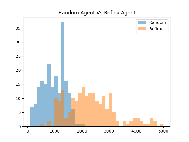
The histogram depicts that the reflex agent on average performs significantly better than the random agent. What is fascinating to note is that even though the agent’s actions are deterministic, the seed of the environment created a large amount of variance in the scores observed. It is arguably misleading to only provide a single score for an agent as its performance because the environment seed has a large impact on the non-random agent’s scores.

Reflex Agent: 
    mean:2385.25
    max:8110.0 
    min:530.0 
    sd:1066.217115553863 
    median:2250.0 
    n:200

Random Agent:
    mean:976.15 
    max:2030.0
    min:110.0 
    sd:425.2712987023695 
    median:980.0 
    n:200

One thing that is interesting about comparing the two distributions is that the reflex agent has a much larger standard deviation in its scores than the random agent. It is also interesting to note that the reflex agent’s worst performance was significantly better than the random agent’s worst performance. Also, the best performance of the reflex agent shatters the best performance of the random agent.

Random agent vs reflex
F_onewayResult(
    statistic=299.86689786081956, 
    pvalue=1.777062051091977e-50
)

Since we took such a sample size of two hundred, and the populations were significantly different, we got a p score of nearly zero (1.77e-50). With a p-value like this, we can say with nearly 100% confidence (with rounding) that these two populations are different and that the reflex agent out-performs the random agent.

5 Genetic Algorithm

Genetic algorithms employ the same tactics used in natural selection to find an optimal solution to an optimization problem. Genetic algorithms are often used in high dimensional problems where the optimal solutions are not apparent. Genetic algorithms are commonly used to tune the hyper-parameters of a program. However, this algorithm can be used in any scenario where you have a function that defines how well a solution is.

In the scenario of asteroids, we can employ genetic algorithms to find the optimal sequence of moves to make to achieve the highest score possible. The chromosomes are well defined as the sequence of actions to loop through and the fitness function is simply the score that the agent achieves.

5.1 Algorithm Implementation

The actual implementation of the genetic algorithm was pretty straight forward, the agent simply looped through a sequence of events where each event represents a gene on the chromosome.

class Agent(object):
    """Very Basic GA Agent"""
    def __init__(self, action_space, chromosome):
        self.action_space = action_space
        self.chromosome = chromosome
        self.index = 0

    # You should modify this function
    def act(self, observation, reward, done):
        if self.index >= len(self.chromosome)-1:
            self.index = 0
        else:
            self.index = self.index + 1
        return self.chromosome[self.index]

Rather than using a library, a simple home-brewed genetic algorithm was created from scratch. The basic algorithm essentially is in a loop that runs functions necessary to iterate through each generation. Each generation can be broken apart into a few steps:

• selection: removes the worst-performing chromosomes
• mating: uses crossover to create new chromosomes
• mutation: adds randomness to the chromosome
• fitness: evaluates the performance of each chromosome

In roughly 100 lines of python, a basic genetic algorithm was crafted.

AVAILABLE_COMMANDS = [0,1,2,3,4]


def generateRandomChromosome(chromosomeLength):
    chrom = []
    for i in range(0, chromosomeLength):
        chrom.append(choice(AVAILABLE_COMMANDS))
    return chrom


"""
creates a random population
"""
def createPopulation(populationSize, chromosomeLength):
    pop = []
    for i in range(0, populationSize):
        pop.append((0,generateRandomChromosome(chromosomeLength)))
    return pop


"""
computes fitness of population and sorts the array based
on fitness
"""
def computeFitness(population):
    for i in range(0, len(population)):
        population[i] = (calculatePerformance(population[i][1]), population[i][1])
    population.sort(key=lambda tup: tup[0], reverse=True) # sorts population in place


"""
kills the weakest portion of the population
"""
def selection(population, keep):
    origSize = len(population)
    for i in range(keep, origSize):
        population.remove(population[keep])



"""
Uses crossover to mate two chromosomes together.
"""
def mateBois(chrom1, chrom2):
    pivotPoint = randrange(len(chrom1))
    bb = []
    for i in range(0, pivotPoint):
        bb.append(chrom1[i])
    for i in range(pivotPoint, len(chrom2)):
        bb.append(chrom1[i])
    return (0, bb)
    


"""
brings population back up to desired size of population
using crossover mating
"""
def mating(population, populationSize):
    newBlood = populationSize - len(population)

    newbies = []
    for i in range(0, newBlood):
        newbies.append(mateBois(choice(population)[1], 
                                choice(population)[1]))
    population.extend(newbies)


"""
Randomly mutates x chromosomes -- excluding best chromosome
"""
def mutation(population, mutationRate):
    changes = random() * mutationRate * len(population) * len(population[0][1])
    for i in range(0, int(changes)):
        ind = randrange(len(population) -1) + 1
        chrom = randrange(len(population[0][1]))
        population[ind][1][chrom] =  choice(AVAILABLE_COMMANDS)


"""
Computes average score of population
"""
def computeAverageScore(population):
    total = 0.0
    for c in population:
        total = total + c[0]
    return total/len(population)


def runGeneration(population, populationSize, keep, mutationRate):
    selection(population, keep)
    mating(population, populationSize)
    mutation(population, mutationRate)
    computeFitness(population)


"""
Runs the genetic algorithm
"""
def runGeneticAlgorithm(populationSize, maxGenerations, 
                        chromosomeLength, keep, mutationRate):
    population = createPopulation(populationSize, chromosomeLength)

    best = []
    average = []
    generations = range(1, maxGenerations + 1)

    for i in range(1, maxGenerations + 1):
        print("Generation: " + str(i))
        runGeneration(population, populationSize, keep, mutationRate)

        a = computeAverageScore(population)
        average.append(a)
        best.append(population[0][0])

        print("Best Score: " + str(population[0][0]))
        print("Average Score: " + str(a))
        print("Best chromosome: " + str(population[0][1]))
        print()

    pyplot.plot(generations, best, color='g', label='Best')
    pyplot.plot(generations, average, color='orange', label='Average')

    pyplot.xlabel("Generations")
    pyplot.ylabel("Score")
    pyplot.title("Training GA Algorithm")
    pyplot.legend()
    pyplot.show()

5.2 Results

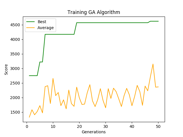
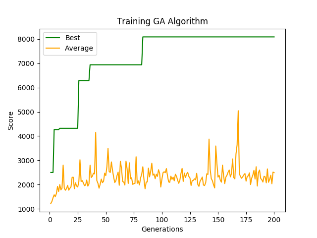
Generation: 200
Best Score: 8090.0
Average Score: 2492.6666666666665
Best chromosome: [1, 4, 1, 4, 4, 1, 0, 4, 2, 4, 1, 3, 2, 0, 2, 0, 0, 1, 3, 0, 1, 0, 4, 0, 1, 4, 1, 2, 0, 1, 3, 1, 3, 1, 3, 1, 0, 4, 4, 1, 3, 4, 1, 1, 2, 0, 4, 3, 3, 0]

It is impressive that a simple genetic algorithm can learn how to perform well when the seed is fixed. When compared to the random agent which had a max score of 3320 with a fixed seed, the optimized genetic algorithm shattered the random agents’ best performance by a factor of 2.5.

Since we trained an optimized set of actions to take to achieve a high score on a specific seed, what would happen if we randomized the seed? A test was conducted to compare the trained GA agent with 200 generations against the random agent. For both agents, the seed was randomized by setting it to the current time.

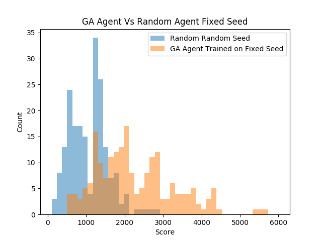
GA Performance Trained on Fixed Seed:
    mean:2257.9 
    max:5600.0
    min:530.0 
    sd:1018.4363455808125 
    median:2020.0 
    n:200

Random Random Seed:
    mean:1079.45 
    max:2800.0 
    min:110.0 
    sd:498.9340612746338 
    median:1080.0 
    n:200

F_onewayResult(
    statistic=214.87432376234608, 
    pvalue=3.289638100969386e-39
)

As expected, the GA agent did not perform as well on random seeds as it did on the fixed seed that it was trained on. However, the GA was able to find an action sequence that statistically beat the random agent as observed in the score distributions above and the extremely small p-value. Although luck was a part of getting the agent to get a score of 8k on the seed of zero, the skill that it learned was somewhat applicable to other seeds. After replaying the video of the agent play, it just slowly drifts around the screen and shoots at asteroids in front of it. This has a major advantage over the random agent since the random agent tends to move very fast and rotate spastically.

5.3 Future Work

This algorithm was more or less a last-minute hack to see if I can make a cool video of a high scoring asteroids agent. Future agents using genetic algorithms would incorporate reflex to dynamically respond to the environment. Based on which direction asteroids are in proximity to the player, the agent could select a different chromosome of actions to execute. This would potentially yield scores above ten thousand if trained and implemented correctly. Future training should also incorporate randomness to the seed so that the skills learned are the most transferable to other random environments.

6 Deep Q-Learning Agent

6.1 Introduction:

The inspiration behind attempting a reinforcement learning agent for this problem scope is the original DQN paper that came out from Deepmind, “Playing Atari with Deep Reinforcement Learning.” This paper showed the potential of utilizing this Deep Q-learning methodology on a variety of simulated Atari games using one standardized architecture across all. Reinforcement learning has always been of interest and to have the opportunity to spend time learning about it while applying for a class setting was exciting, even if it is out of the scope of the class presently. It has been an exciting challenge to read through and implement a research paper to get similar results.

Deep Q-Learning is an extension of the standard Q-Learning algorithm in which a neural network is used to approximate the optimal action-value function, Q*(s,a). The action-value function is the function that outputs the expected maximum reward given a state and a policy mapping to actions or distributions of actions. Logically, this works as the Q function follows the Bellman equation identity, which states that if the optimal action for the next step state is known, then the optimal output given an action a’ follows by maximizing the expected reward of the equation, r+Q*(s’,a’). Thus, the reinforcement learning part comes in the form of a neural network approximating the optimal action-value function by using the Bellman equation identity as an iterative update at every time step.

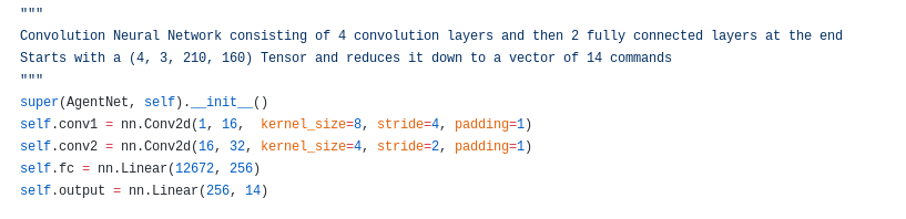
6.2 Agent architecture:

The basis of the network architecture is a basic convolutional network with 2 conv layers, a fully connected layer, and then an output layer of 14 classes with each representing an individual action. The first layer consists of 16 8x8 filters and takes a stride 4 while the second has 32 4x4 filters and only takes a stride of 2. Following this layer, the filters are compressed into a 1-D representation vector of size 12,672 that’s passed through a fully connected layer of 256 nodes.

All layers sans the output layer are activated using the ReLU function. The optimization algorithm of choice was the Adam optimizer, using a learning rate equal to .0001 and default betas of [.9, .99]. The discount factor, or gamma, related to future expected rewards was set at .99 and the probability of taking a random action per action step was linearly annealed from 1.0 down to a fixed .1 after one million seen frames.

6.3 Experience Replay:

One of the main points within the original paper that significantly helped the training of this network is the introduction of a Replay Buffer that is used during the training. To break all the temporal correlation between sequential frames and biasing the training of a network-based off certain chains of situations, a historical buffer of transitions is used to sample mini-batches to train on per time step. Every time an action is made, a tuple consisting of the current state, the action is taken, the reward gained, and the subsequent state (s, a, r, s’) is stored into the buffer. And at every training step, a mini-batch is sampled from the buffer and used to train the network. This allows the network to be trained in non-correlated transitions and hopefully train in a more generalized way to the environment rather than biased to a string of similar actions.

6.4 Preprocessing:

One of the first issues that had to be tackled was the issue of the high dimensionality of the input image and how that information was duplicated stored in the Replay Buffer. Each observation given from the environment is a matrix of (210, 160, 3) pixels representing the RGB pixels within the frame. For time and being computationally efficient, it was needed to preprocess and reduce the dimensionality of the observations as a single frame stack (of which there are two per transition) consists of (4, 3, 210, 160) or 403,000 input features that would have to be dealt with.

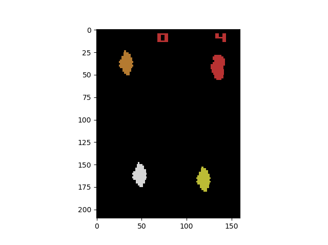
Firstly, images are converted into a grayscale image and the reward/number lives section at the top of the screen is cut out since it is irrelevant to the network’s vision. Furthermore, the now (4, 192, 160) matrix was downsampled by taking every other pixel to (4, 96, 80), resulting in a change from 403,000 input features to only 30,720 - a substantial reduction in the calculations needed while maintaining strong input information for the network.

6.5 Training:

Training for the bot was conducted by modifying the main function to allow games to immediately start after one was finished, to make continuous training of the agent easier. All the environment parameters were reset and the temporary attributes of the agent (ie. current state/next state) were flushed. For the first four frames of a game, the bot just gathered a stack of frames. And following that, at every time the next state was compiled and the transition tuple pushed onto the buffer, as well as a training step for the agent. For the training step, a random batch was grabbed from the replay buffer and used to calculate the loss function between actual and expected Q-values. This was used to calculate the gradients for the backpropagation of the network.

6.6 Outcome:

Unfortunately, the result of 48 hours of continuous training, 950 games played, and roughly 1.3 million frames of game footage seen, was that the agent converged to a suicidal policy that resulted in a consistent garbage performance.

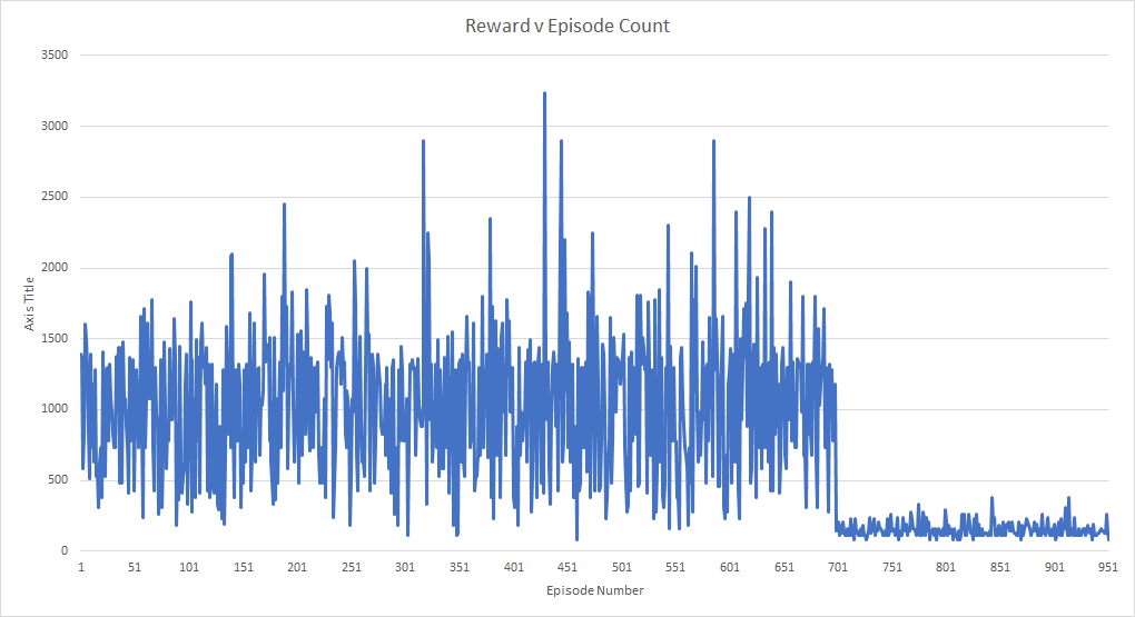
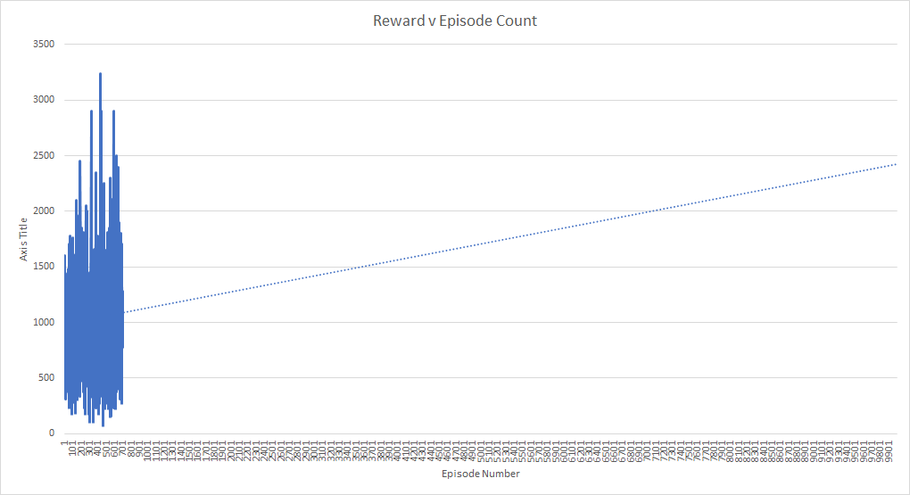
The model transitioned to the fixed 90% model action chance around episode 700, which is exactly where the agent starts to go awry. The strange part about this is since the random action chance is linearly annealed over the first million frames, if the agent had continuously been following a garbage policy, it would’ve been expected that the rewards would steadily decrease over time as the network takes more control.

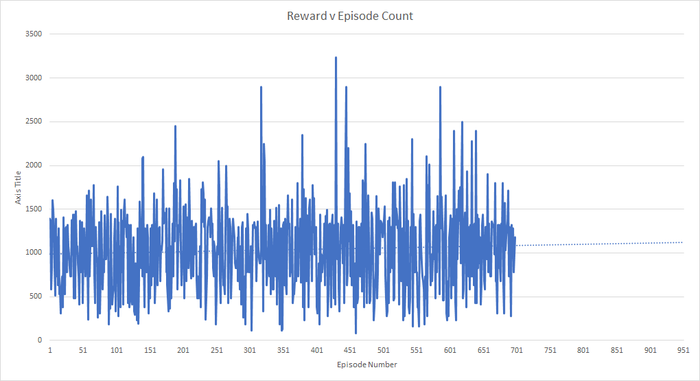
Up until that point, the projection of the reward trendline was a steady rise per the number of episodes. Expanding this out until 10,000 frames (approximately 10 million frames seen, the same amount of time the original Deepmind paper trained these bots for), the projected score is in the realms of 2,400 to 2,500 - which matches up closely to the well-tuned reflex agent and the GA agent on a random seed.

It would’ve been exciting to see how the model compared to our reflex agent had it been able to train consistently up until the end.

6.7 Limitations:

There were a fair number of limitations that were present within the execution and training of this model that possibly contributed to the slow and unstable training of the network. Differences in the algorithm from the original paper is that the optimization function utilized was the Adam optimizer instead of RMSProp and the replay buffer only took into consideration the previous 50k frames, not the past one million. It might be possible that the weaker replay buffer was to blame as the model was continuously fed a sub-optimal within its past 50,000 frames that caused it to diverge so heavily near the end.

One issue in preprocessing that might’ve led the bot astray is using not using the max pixelwise combination between sequential frames in order to have each frame include both the asteroids and the player. Since the Atari (and by extension, this environment simulation) doesn’t render the asteroids and the player sprite all in the same frame, it is possible that the network was unable to extract any coherent connection between the alternating frames.

Regarding optimizations built on the DQN algorithm past the original Deepmind paper, we did not use a policy and a target network in training. In the original algorithm, the estimation and attempt at converging to the target policy is unstable due to the target network’s weights continuously shifting during training. For the network, it’s hard to converge to something that’s continually shifting at every time step and leads to very noisy and unstable training. One optimization that has been proposed for DQN is to have a policy and target network. At every timestep, the policy network’s weights are updated with the calculated gradients while the target network is maintained for a number of steps. This lets the target policy be still for a few time steps while the network is converging to it and leads to more stable and guided training.

Perhaps the largest limitation in training was the computational power used for training. The network was trained on a single GTX1060ti GPU, which led to just single episodes taking a few minutes to complete. It would’ve taken an incredibly long time to hit 10 million seen frames as even just 1.3 million took approximately 48 hours. It’s probable that our implementation is inefficient in its calculations, however it is a well known limitation of RL that it is time and computationally intensive.

6.8 Deep Q Conclusions:

This was a fun agent and algorithm to implement, even if at present it has given little to no results back in terms of performance. The plan is to continue testing and training the agent, even after the deadline. Reinforcement learning is a complicated and hard to debug environment, but similarly an exciting challenge due to its potential for solving and overcoming problems.

7 Conclusion

This project demonstrated how fun it can be to train AI agents to play video games. Although none of our agents are earth-shatteringly amazing, we were able to use statistical measures to determine that the reflex and GA agents outperformed the random agent. The GA agent and the convolutional neural network show very promising and future work can be used to drastically improve their results.