Shallow Dive into Open CV
Sun Feb 23 2020
This blog post going over the basic image manipulation things you can do with Open CV. Open CV is an open-source library of computer vision tools. Open CV is written to be used in conjunction with deep learning frameworks like TensorFlow. This tutorial is going to be using Python3, although you can also use Open CV with C++, Java, and Matlab
1 Reading and Displaying Images
The first thing that you want to do when you start playing around with open cv is to import the dependencies required. Most basic computer vision projects with OpenCV will use NumPy and matplotlib. All images in Open CV are represented as NumPy matrices with shape (x, y, 3), with the data type uint8. This essentially means that every image is a 2d matrix with three color channels for BGR where each pixel can have an intensity between 0 and 255. Zero is black where 255 is white in grayscale.
# Open cv library
import cv2

# numpy library for matrix manipulation
import numpy as np

# matplotlib for displaying the images
from matplotlib import pyplot as plt
Reading an image is as easy as using the “cv2.imread” function. If you simply try to print the image with Python’s print function, you will flood your terminal with a massive matrix. In this post, we are going to be using the infamous Lenna image which has been used in the Computer Vision field since 1973.
lenna = cv2.imread('lenna.jpg')

# Prints a single pixel value
print(lenna[50][50])

# Prints the image dimensions
# (width, height, 3 -- BRG)
print(lenna.shape)
[ 89 104 220]
(440, 440, 3)By now you might have noticed that I am saying “BRG” instead of “RGB”; in Open CV colors are in the order of “BRG” instead of “RGB”. This makes it particularly difficult when printing the images using a different library like matplotlib because they expect images to be in the form “RGB”. Thankfully for us we can use some functions in the Open CV library to convert the color scheme.
def printI(img):
    rgb = cv2.cvtColor(img, cv2.COLOR_BGR2RGB)
    plt.imshow(rgb)

printI(lenna)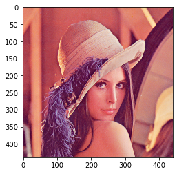
Going a step further with image visualization, we can use matplotlib to view images side by side to each other. This makes it easier to make comparisons when running different algorithms on the same image.
def printI3(i1, i2, i3):
    fig = plt.figure()
    ax1 = fig.add_subplot(1,3,1)
    ax1.imshow(cv2.cvtColor(i1, cv2.COLOR_BGR2RGB))
    ax2 = fig.add_subplot(1,3,2)
    ax2.imshow(cv2.cvtColor(i2, cv2.COLOR_BGR2RGB))
    ax3 = fig.add_subplot(1,3,3)
    ax3.imshow(cv2.cvtColor(i3, cv2.COLOR_BGR2RGB))


def printI2(i1, i2):
    fig = plt.figure()
    ax1 = fig.add_subplot(1,2,1)
    ax1.imshow(cv2.cvtColor(i1, cv2.COLOR_BGR2RGB))
    ax2 = fig.add_subplot(1,2,2)
    ax2.imshow(cv2.cvtColor(i2, cv2.COLOR_BGR2RGB))
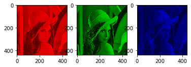
If we zero out the other colored layers and only left one channel, we can visualize each channel individually. In the following example notice that image.copy() generates a deep-copy of the image matrix – this is a useful NumPy function.
def generateBlueImage(image):
    b = image.copy()
    # set the green and red channels to 0
    # note images are in BGR
    b[:, :, 1] = 0
    b[:, :, 2] = 0
    return b


def generateGreenImage(image):
    g = image.copy()
    # sets the blue and red channels to 0
    g[:, :, 0] = 0
    g[:, :, 2] = 0
    return g

def generateRedImage(image):
    r = image.copy()
    # sets the blue and green channels to 0
    r[:, :, 0] = 0
    r[:, :, 1] = 0
    return r

def visualizeRGB(image):
    printI3(generateRedImage(image), generateGreenImage(image), generateBlueImage(image))
visualizeRGB(lenna)
2 Grayscale Images
Converting a color image to grayscale reduces the dimensionality because you are squishing each color layer into one channel. Open CV has a built-in function to do this.
glenna = cv2.cvtColor(lenna, cv2.COLOR_BGR2GRAY)
printI(glenna)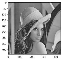
The builtin function works in most applications, however, you sometimes want more control in which color layers are weighted more in generating the grayscale image. To do that you can
def generateGrayScale(image, rw = 0.25, gw = 0.5, bw = 0.25):
    """
    Image is the open cv image
    w = weight to apply to each color layer
    """
    w = np.array([[[ bw, gw,  rw]]])
    gray2 = cv2.convertScaleAbs(np.sum(image*w, axis=2))
    return gray2
printI(generateGrayScale(lenna))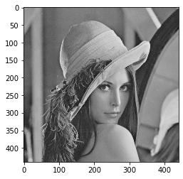
Notice that the sum of the weights is equal to 1 if it above 1, it would brighten the image but if it was below 1, it would darken the image.
printI2(generateGrayScale(lenna, 0.1, 0.3, 0.1), generateGrayScale(lenna, 0.5, 0.6, 0.5))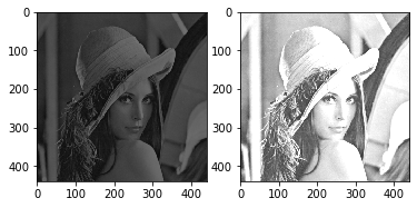
We could also use our function to display the grayscale output of each color layer.
printI3(generateGrayScale(lenna, 1.0, 0.0, 0.0), generateGrayScale(lenna, 0.0, 1.0, 0.0), generateGrayScale(lenna, 0.0, 0.0, 1.0))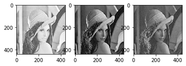
Based on this output, the red layer is the brightest which makes sense because the majority of the image is in a pinkish/red tone.
3 Pixel Operations
Pixel operations are simply things that you do to every pixel in the image.
3.1 Negative
To take the negative of an image, you simply invert the image. Ie: if the pixel was 0, it would now be 255, if the pixel was 0 it would now be 255. Since all the images are unsigned ints of length 8, right once, a pixel hits a boundary, it would automatically wrap over which is convenient for us. With NumPy, if you subtract a number from a matrix, it would do that for every element in that matrix – neat. Therefore if we wanted to invert an image we could just take 255 and subtract it from the image.
invert_lenna = 255 - lenna
printI(invert_lenna)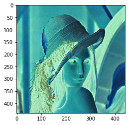
3.2 Darken And Lighten
To brighten and darken an image you can add constants to the image because that would push the image closer twords 0 and 255 which is black and white.
bright_bad_lenna = lenna + 25

printI(bright_bad_lenna)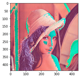
Notice that the image got brighter but in some parts the image got inverted. This is because when we add two images, and we don’t want to wrap, we have to set a clipping threshold to be the 0 and 255. IE: when we add a constant to the image at pixel 240, we don’t want it to wrap back to 0, we just want it to retain a value of 255. Open CV has built-in functions for this.
def brightenImg(img, num):
    a = np.zeros(img.shape, dtype=np.uint8)
    a[:] = num
    return cv2.add(img, a)

def darkenImg(img, num):
    a = np.zeros(img.shape, dtype=np.uint8)
    a[:] = num
    return cv2.subtract(img, a)

brighten_lenna = brightenImg(lenna, 50)
darken_lenna = darkenImg(lenna, 50)

printI2(brighten_lenna, darken_lenna)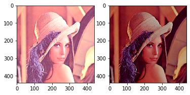
3.3 Contrast
Adjusting the contrast of an image is a matter of multiplying the image by a constant. Multiplying by a number greater than 1 would increase the contrast and multiplying by a number lower than 1 would decrease the contrast.
def adjustContrast(img, amount):
    """
    changes the data type to float32 so we can adjust the contrast by
    more than integers, then we need to clip the values and
    convert data types at the end.
    """
    a = np.zeros(img.shape, dtype=np.float32)
    a[:] = amount
    b = img.astype(float)
    c = np.multiply(a, b)
    np.clip(c, 0, 255, out=c) # clips between 0 and 255
    return c.astype(np.uint8)
printI2(adjustContrast(lenna, 0.8) ,adjustContrast(lenna, 1.3))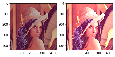
4 Noise
I most cases you don’t want to add random noise to your image, however, in some algorithms, it becomes necessary to do for testing. Noise is anything that makes the image imperfect. In the “real world” this is usually in the form of dead pixels on your camera lens or other things distorting your view.
4.1 Salt and Pepper
Salt and pepper noise is adding random black and white pixels to your image.
import random

def uniformNoise(image, num):
    img = image.copy()
    h, w, c = img.shape
    x = np.random.uniform(0,w,num)
    y = np.random.uniform(0,h,num)

    for i in range(0, num):
        r = 0 if random.randrange(0,2) == 0 else 255
        img[int(x[i])][int(y[i])] = np.asarray([r, r, r])

    return img
printI2(uniformNoise(lenna, 1000), uniformNoise(lenna, 7000))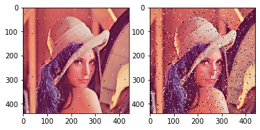
5 Image Denoising
It is possible to remove the salt and pepper noise from an image to clean it up. Unlike how my professor worded it, this is not “enhancing” the image, this is merely using filters that remove the noise from the image by blurring it.
5.1 Moving Average
The moving average technique sets each pixel equal to the average of its neighborhood. The bigger your neighborhood the more the image is blurred.
bad_lenna = uniformNoise(lenna, 6000)

blur_lenna = cv2.blur(bad_lenna,(3,3))

printI2(bad_lenna, blur_lenna)
As you can see, most of the noise was removed from the image but, imperfections were left. To see the effects of the filter size, you can play around with it.
blur_lenna_3 = cv2.blur(bad_lenna,(3,3))
blur_lenna_8 = cv2.blur(bad_lenna,(8,8))
printI2(blur_lenna_3, blur_lenna_8)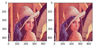
5.2 Median Filtering
Median filters transform every pixel by taking the median value of its neighborhood. This is a lot better than average filters for noise reduction because it has less of a blurring effect and it is extremely well at removing outliers like salt and pepper noise.
median_lenna = cv2.medianBlur(bad_lenna,3)

printI2(bad_lenna, median_lenna)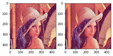
6 Remarks
Open CV is a vastly powerful framework for image manipulation. This post only covered some of the more basic applications of Open CV. Future posts might explore some of the more advanced techniques in computer vision like filters, Canny edge detection, template matching, and Harris Corner detection.
Recent Posts
My Wall Mounted Raspberry Pi HomelabThe Data Spotify Collected On Me Over Ten Years
Visualizing Fitbit GPS Data
Running a Minecraft Server With Docker
DIY Video Hosting Server
Running Scala Code in Docker
Quadtree Animations with Matplotlib
2020 in Review
Segmenting Images With Quadtrees
Implementing a Quadtree in Python