Creating Pixel Art With Open CV

Mon Jun 29 2020

Let’s jump right into the fun and start making pixel art with Open CV. Before you read this article, consider checkout out these articles:

• Shallow Dive into Open CV
• Image Clustering with K-means

Like most CV projects, we need to start by importing some libraries and loading an image.

# Open cv library
import cv2

# matplotlib for displaying the images 
from matplotlib import pyplot as plt

img = cv2.imread('dolphin.jpg')

I like to define scripts to print images nicely in a Jupyter notebook.

def printI(img):
    rgb = cv2.cvtColor(img, cv2.COLOR_BGR2RGB)
    plt.imshow(rgb)
    
def printI2(i1, i2):
    fig = plt.figure()
    ax1 = fig.add_subplot(1,2,1)
    ax1.imshow(cv2.cvtColor(i1, cv2.COLOR_BGR2RGB))
    ax2 = fig.add_subplot(1,2,2)
    ax2.imshow(cv2.cvtColor(i2, cv2.COLOR_BGR2RGB))
    
printI(img)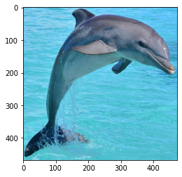

To pixelate an image, we can use the open cv resize function. To make the image viewable, after we shrink the picture, we resize it again to be the size of the original image.

def pixelate(img, w, h):
    height, width = img.shape[:2]

    # Resize input to "pixelated" size
    temp = cv2.resize(img, (w, h), interpolation=cv2.INTER_LINEAR)

    # Initialize output image
    return cv2.resize(temp, (width, height), interpolation=cv2.INTER_NEAREST)

img16 = pixelate(img, 16, 16)

printI2(img, img16)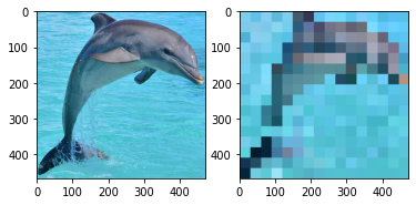

We can try a few different shrinkage sizes. 32x32 seems to work the best.

img32 = pixelate(img, 32, 32)
img64 = pixelate(img, 64, 64)

printI2(img32, img64)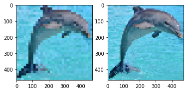

img8 = pixelate(img, 8, 8)
printI(img8)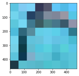

Despite the images being pixelated, they have imperfections that normal pixel art wouldn’t have. To remove the noise and make it look smoother, we will do k-means clustering on the pixelated images. K-means will reduce the number of colors in the image and eliminate any noise. Most of the clustering code is from my blog post: Image Clustering with K-means

import skimage
from sklearn.cluster import KMeans
from numpy import linalg as LA
import numpy as np

def colorClustering(idx, img, k):
    clusterValues = []
    for _ in range(0, k):
        clusterValues.append([])
    
    for r in range(0, idx.shape[0]):
        for c in range(0, idx.shape[1]):
            clusterValues[idx[r][c]].append(img[r][c])

    imgC = np.copy(img)

    clusterAverages = []
    for i in range(0, k):
        clusterAverages.append(np.average(clusterValues[i], axis=0))
    
    for r in range(0, idx.shape[0]):
        for c in range(0, idx.shape[1]):
            imgC[r][c] = clusterAverages[idx[r][c]]
            
    return imgC

def segmentImgClrRGB(img, k):
    
    imgC = np.copy(img)
    
    h = img.shape[0]
    w = img.shape[1]
    
    imgC.shape = (img.shape[0] * img.shape[1], 3)
    
    #5. Run k-means on the vectorized responses X to get a vector of labels (the clusters); 
    #  
    kmeans = KMeans(n_clusters=k, random_state=0).fit(imgC).labels_
    
    #6. Reshape the label results of k-means so that it has the same size as the input image
    #   Return the label image which we call idx
    kmeans.shape = (h, w)

    return kmeans

def kMeansImage(image, k):
    idx = segmentImgClrRGB(image, k)
    return colorClustering(idx, image, k)

printI(kMeansImage(img, 5))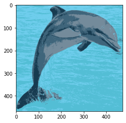

Running the k-means algorithm on the 32x32 bit image produces a cool look.

printI(kMeansImage(img32, 3))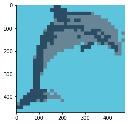

We can compare the original, pixelated, and clustered images side by side.

def printI3(i1, i2, i3):
    fig = plt.figure(figsize=(18,6))
    ax1 = fig.add_subplot(1,3,1)
    ax1.imshow(cv2.cvtColor(i1, cv2.COLOR_BGR2RGB))
    ax2 = fig.add_subplot(1,3,2)
    ax2.imshow(cv2.cvtColor(i2, cv2.COLOR_BGR2RGB))
    ax3 = fig.add_subplot(1,3,3)
    ax3.imshow(cv2.cvtColor(i3, cv2.COLOR_BGR2RGB))
    plt.savefig('trifecta.png')
printI3(img, img32, kMeansImage(img32, 3))